Connect the Dots: Sampling From Diffusion Models (DDMs)

How to Generate Novel Samples Using Denoising Diffusion Models (DDMs).

Sep 06, 2023

Table of Content

Introduction.
The Sampling Equation: The Brilliant Math Behind DDMs Sampling.
The Standard Sampling Algorithm: Decode Math Using the Algorithm Language.
Why the Standard Sampling Algorithm doesn't work in Practice?
The Antidote: The Stride Sampling Algorithm.
Putting it All Together.
Recap.
References.

1. Introduction

Today, we will discover the last missing piece in our puzzle before implementing the Denoising Diffusion Model (DDM) from scratch! As we can see in our previous post, we discussed the reverse process in diffusion models. We explained the general idea behind the reverse process, and we learned that the distribution:

\(q(x_t | x_{t-1}) = \mathcal{N}(x_t | \sqrt {1-\beta_t} x_{t-1} , \beta_t I)\)

can't be learned directly, and we have to approximate it using a neural network, UNet. Also, we knew that the objective function of UNet is simplified to the standard MSE loss:

\(L(\epsilon_t, \epsilon_\theta) = E_{t\sim[1:T]x_0, \epsilon_t}\left[ \|\epsilon_t - \epsilon_\theta(\sqrt{\bar \alpha_t} \space x_{0} + \sqrt{1- \bar \alpha_t} \space \epsilon_t, t)\|^2 \right] \)

Leaving the full process of the derivation of that objective function to another post. Finally, we covered the building blocks of UNet, and we learned that the network receives a noise rate and noisy input, and it tries to predict the amount of noise inside that sample.

In this post, we will be discussing how we can generate or sample from diffusion models. Sampling from diffusion models is really a unique process compared to other deep learning architectures like GAN and VAE. We will cover the math behind the sampling process, and then we will learn how we can translate that math into a coding algorithm.

After that, we will know why that algorithm doesn't work in practice. And, how a simple trick-the stride sampling-can speed up the diffusion computation. So, without further ado, let's get started!

2. The Brilliant Math Behind DDMs Sampling

The sampling from diffusion models is iteratively performed through this equation:

\(x_{t-1} = \sqrt{\bar \alpha_{t-1}}(\frac{x_t - \sqrt{1-\bar\alpha_t}.\epsilon_\theta^{(t)}(x_t)}{\sqrt{\bar \alpha_t}}) + \sqrt{1-\bar\alpha_{t-1}-\sigma_t}.\epsilon_\theta^{(t)}(x_t)+\alpha_t\epsilon_t\)

Yes! It is a giant equation but trust me it is very simple to grasp. To fully understand this equation, let's break it and discuss each term.

2.1 [1st Term]: Remove the Noise

2.1.1 The Estimated Input Sample Term

\(x_0\equiv (\frac{x_t - \sqrt{1-\bar\alpha_t}.\epsilon_\theta^{(t)}(x_t)}{\sqrt{\bar \alpha_t}})\)

The first term of our equation is the estimated value of our real input sample. This term represents the closest estimate to the real input sample x0. If we recall the forward process equation we discussed earlier, we can notice this term is the same but with some rearrangements. Here is the forward process equation:

\(x_t = \sqrt{\bar \alpha_t}.x_0 - \sqrt{1-\bar\alpha_t}.{\epsilon}\)

And here is our equation after the re-arrangement:

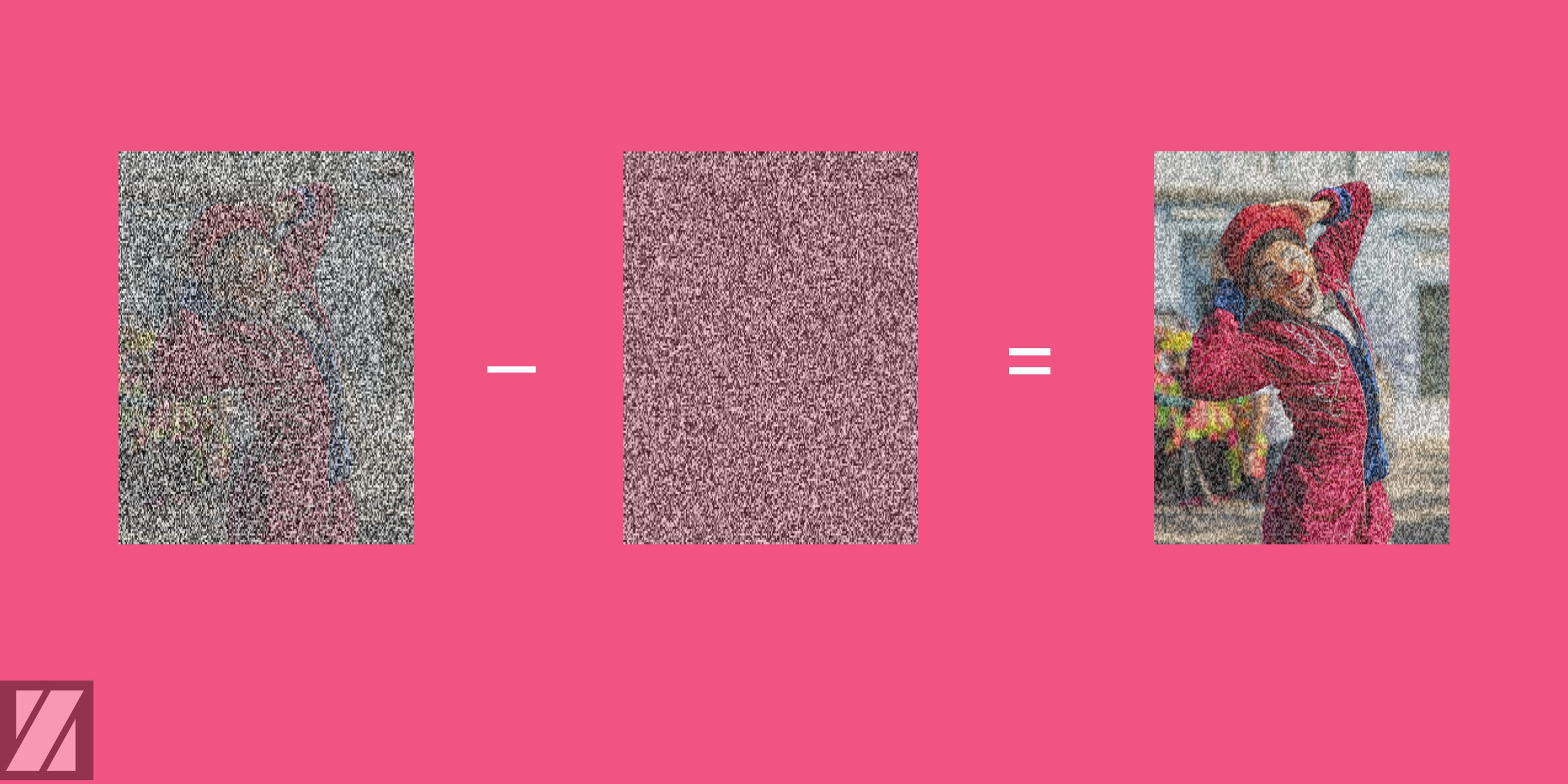
\(x_t = \sqrt{\bar \alpha_t}.x_0 - \sqrt{1-\bar\alpha_t}.\underbrace{\textcolor{red}{\epsilon_\theta^{(t)}}(x_t)}_{\text{predicted by UNet.}}\)

As we can see, the only difference between this equation, and the forward process question is that the noise is predicted in this case by the UNet model.

2.1.2 The Estimated Noise Term

\( \tilde \epsilon_{t-1} = \epsilon_\theta^{(t)}(x_t)\)

This term represents the total noise predicted by our network, UNet at time-step t.

2.1.3 The Estimated Noisy Sample at (t-1) Term

\(\tilde x_{t-1}\equiv \frac{x_t - \sqrt{1-\bar\alpha_t}.\epsilon_\theta^{(t)}(x_t)}{\sqrt{\bar \alpha_t}} + \epsilon_\theta^{(t)}(x_t)\)

If we add the total noise in section 2.1.2 to the estimated input sample x0 in section 2.1.1, we would get an estimate of the noisy input sample at step = t-1.

2.1.4 The Scaled Estimated Noisy Sample at (t-1) Term

\(x_{t-1}^{scaled} = \textcolor{red}{\sqrt{\bar \alpha_{t-1}}}(\frac{x_t - \sqrt{1-\bar\alpha_t}.\epsilon_\theta^{(t)}(x_t)}{\sqrt{\bar \alpha_t}}) - \textcolor{red}{\sqrt{1-\bar\alpha_{t-1}-\sigma_t}}.\epsilon_\theta^{(t)}(x_t)\)

This term will balance the equation a little bit. As we can see, we scaled the real input sample estimate x0 and the predicted noise at time step = t-1 with some factors. These factors ensure that our final estimation of the noisy input sample at t-1 will have a unit variance, which helps us to continue the sampling process.

Specifically, the second term ensures that predicted noise by UNet will be normalized or adapted by the values of variances from time-step t = 0, till t= t-1.

If we don’t normalize this predicted noise, the condition of always having a unit Gaussian noise at each time step will break, which is necessary for the sampling process.

2.2 [2nd Term]: Control the Sampling: Random Generation Factor

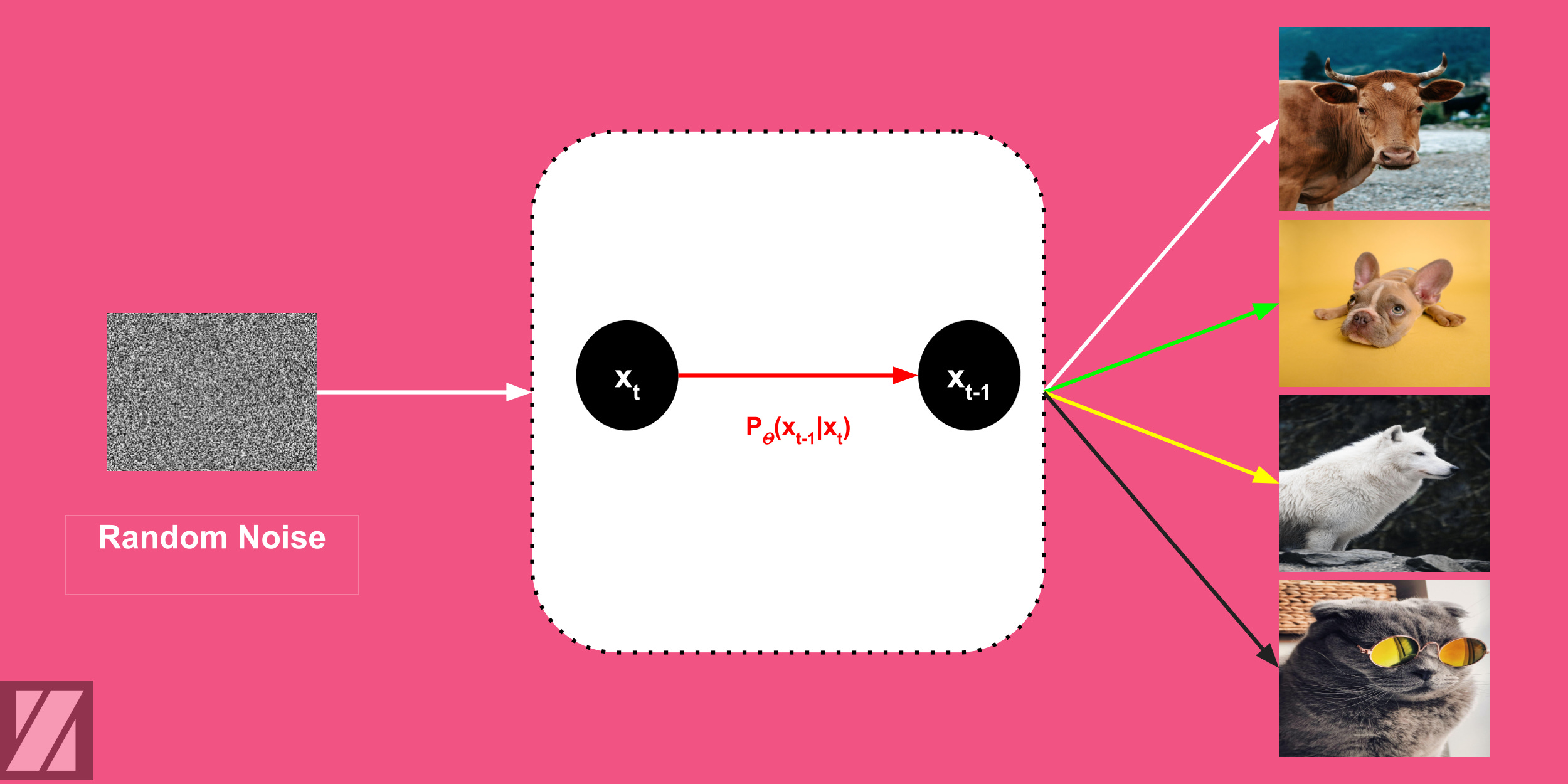
The same random noise leads to different samples.

\(x_{t-1} = \textcolor{red}{\sqrt{\bar \alpha_{t-1}}}(\frac{x_t - \sqrt{1-\bar\alpha_t}.\epsilon_\theta^{(t)}(x_t)}{\sqrt{\bar \alpha_t}}) - \textcolor{red}{\sqrt{1-\bar\alpha_{t-1}-\sigma_t}}.\epsilon_\theta^{(t)}(x_t)+ \textcolor{blue}{\alpha_t\epsilon_t}\)

This term is used to make the sampling process from the diffusion stochastic. It means a random noise will produce a different sample each time it is processed by the network.

3. The Standard Sampling Algorithm

Let’s see how this equation works in practice:

Sample Generation in Diffusion Models using T = 3.

Let’s take the next example to understand the sampling algorithm. Suppose that we have a diffusion model, and we want to generate a novel image from it. We have credits for using the model over just 3 steps (T= 3), given some random noise.

First, The sampling algorithm starts with predicting the amount of noise in the noise input using the UNet model. This represents the total amount of noise that has been added to an image from t= 0 to t = T = 3.
Second, we find an estimate of the real image using our noise prediction from the previous step using a simple calculation. This represents an estimate of the image at time t= 0.
Third, we will add the predicted noise to this image estimate using a sequential process (F) starting from t = 0 till t = T-1.
Again, we will use our model to predict the total amount of noise at t= T-1, and estimate the real image at t =0.
We will continue this process till the model predicts the total amount of noise at t = 0 and calculate an estimate of the image at t =0. In this stage, the predicted image is considered the final clean image.

4. Why the Standard Sampling Algorithm Doesn't Work in Practice

As we can see, this algorithm is computationally expensive, because, at each time-step t, we need to execute the forward process t-1 steps. This means, in the worst-case scenario when t = n, our algorithm could take a quadratic time:

\(O(n^2)\)

This quadratic time is terrible, especially because each time step involves executing UNet to get the noise predictions.

5. The Stride Sampling Algorithm

How can we optimize this time complexity and make it less expensive?

One simple trick by [Nichol et al.] is to use a non-uniform stride sampling technique. In this sampling, we just skip some time steps rather than going through all the steps to estimate our samples.

7. Recap

In this post, we explored the sampling operation in Denoising Diffusion Models (DDMs).
The sampling equation involves multiple terms, including noise removal, estimated input sample, estimated noise, and scaled estimated noisy sample.
The second term introduces random noise, making the sampling process stochastic.
We explained the standard sampling algorithm, which involves predicting noise, estimating the real image, and adding noise sequentially.
However, the standard algorithm is computationally expensive, with a worst-case quadratic time complexity.
The Stride Sampling Algorithm, a simple optimization technique, skips some time steps to reduce computation time.
In our next post, we will be exploring some complementary topics before implementing the denoising diffusion model from scratch. Stay Tuned!

8. References

Jonathan Ho, Ajay Jain, and Pieter Abbeel. "Denoising Diffusion Probabilistic Models" (2020).
Alex Nichol and Prafulla Dhariwal. "Improved Denoising Diffusion Probabilistic Models" (2021).
David Foster's "Generative Deep Learning, 2nd Edition" (2023).
Weng, Lilian. What are diffusion models? Lil’Log. https://lilianweng.github.io/posts/2021-07-11-diffusion-models/ (Jul 2021).

Before Goodbye!

Want to Cite this Article?

@article{khamies2023connect,
  title   = "Connect the Dots: Sampling From Diffusion Models (DDMs)",
  author  = "Waleed Khamies",
  journal = "Zitoon.ai",
  year    = "2023",
  month   = "Sept",
  url     = "https://publication.zitoon.ai/connect-the-dots-sampling-from-diffusion-models"
}

New to this Series?

New to the “Generative Modeling Series”? Here you can find the previous articles in this series [link to the full series].

Any oversights in this post?

Please report them through this Feedback Form, we really appreciate that!

Thank you for your reading!

We appreciate your reading! If you would like to receive the following posts in this series in your email, please feel free to subscribe to the ZitoonAI Newsletter. Come and Join the Family!