

Denoising Diffusion Models (DDMs) under the Microscope
Introduction to the What(s) & Why(s).


Table of Contents
Introduction.
Why diffusion models?
The Journey From the Source to the Mouth.
Architecture.
Components In Details
Recap.
References
Next Steps.
1. Introduction
Generative models have evolved in the last few years to allow many creative applications (virtual avatars, animation production, video generation, …, etc.) to be adopted by different industries. This advancement is a result of the great research contributions that have been conducted by the people in this field in developing powerful and robust algorithms and techniques.
There is a key algorithm that plays a main role in this advancement and pushing the generative models to the next levels. It allowed the production of realistic images and videos that sometimes it would be hard for the bare eyes to notice the difference.
The Denoising Diffusion Model -also known as Diffusion Models- is a class of generative modeling algorithms that try to learn the distribution of data and provide an efficient approach to sample from this learned distribution.
1.1 The Name: Diffusion
The name diffusion comes from the diffusion phenomena in the thermodynamics field. In thermodynamics, diffusion refers to the movement of particles in a system due to the difference in concentration or energy inside this system. According to Wikipedia, Diffusion is:
the net movement of anything (for example, atoms, ions, molecules, energy) generally from a region of higher concentration to a region of lower concentration
1.2 Diffusion and Deep Learning
In the deep learning field, [Sohl-Dickstein et al] is considered one of the pioneer works that try to connect the diffusion in thermodynamics to the deep learning field. They developed an approach that simultaneously achieves both flexibility and traceability in modeling complex datasets by systematically and slowly destroying the structure in a data distribution through an iterative forward diffusion process. Then, they learn a reverse diffusion process that restores that structure in the data.
1.3 Diffusion Models and Score-Based Models
Diffusion models are built on a well-known class of generative modeling algorithms called score-based generative models (SGMs), which is an energy-based generative modeling algorithm that tries to directly model the data distribution by learning the gradient of the log-likelihood of the data distribution.
The key differences between score-based generative models (SGMs) and diffusion models (DDMs) lie mostly in the modeling and generation stages. In the modeling stage, SGMs learn to model the distribution of data directly p(x), while DDMs learn to model the data generation through a denoising process.
In the generation stage, SGMs use gradient-based methods like Markov Chain Monte Carlo (MCMC) for the sampling process. These methods perform badly when it comes to the generation of high-dimensional data. (i.e. 64x64 images). On the other hand, DDMs apply a denoising process on a Gaussian noise to produce the final sample.
To work around the inefficiency of the sampling in the score-based models, the concepts of the forward process and backward process were introduced in [Song et al]. They use differential equations to move the data to noise and reverse that noise back to the original data. These processes are the backbone of the working of diffusion models.


2. Why Diffusion Models?
Previous generative modeling algorithms suffer from several problems that make them insufficient when it comes to generation quality and performance scalability. For example, VAE models usually fail when it comes to generating high-quality samples, they are prone to low-quality sample production. On the contrary, energy-based models suffer from a slow inference in the generation stage. We can summarize the advantages of diffusion models in the following points:
Samples Quality: DDMs produce high-quality samples that are visually coherent and consistent.
Inference Time: DDMs use the reverse process to generate the samples. This process is much better and time-efficient compared to the previous energy-based methods.
Manipulation: DDMs give more degree of freedom when it comes to manipulation and producing novel samples. We can apply different operations on a Gaussian noise (i.e. arithmetic operations, interpolation, …, etc.), and then give that to the reverse process component to produce a very novel sample.
3. Diffusion Trip: How does the diffusion model generate a novel sample?
Let’s say that we want to use a diffusion model to generate a novel image like the cool Pop Francis image here:
First, we generate a random noise from a standard Gaussian distribution.
Second, starting from time t = T, we feed this noise to a model (R) to predict the total amount of noise: This represents the total amount of noise that has been added to an image from t= 0 till t = T.
Third, we find the noisy Image using our model’s noise prediction from the previous step through a simple calculation. This represents an estimate of the image at time t= 0.
Then, we will add the predicted noise to this image estimate using a sequential process (F) starting from t = 0 till t = T-1.
Again, we will use our model to predict the total amount of noise at t= T-1, and the image at t =0.
We will continue this process till the model predicts the total amount of noise at t = 0 and an estimate of the image at t =0. In this stage, the predicted image is considered as the desired clean image sample.
Here is a visual illustration that explains the previous steps:

4. Architecture

The diffusion model architecture consists of two main components:
Forward Process: This is a non-trainable component that uses a sequential process to perturb an input sample with standard Gaussian noise over multiple steps T.
Reverse Process: This is a trainable component that predicts the amount of noise in a given perturbed input. Some people consider the reverse process components responsible for providing a predicted image besides the noise prediction. However, the predicted image is produced using a constant operation, and not by the trained model.
5. Components In Details
The standard architecture of the Denosing Diffusion Model (DDM) consists of a forward process component and a reverse process component.
The forward process component is a non-trainable element that does not have its weights updated during the training process. Conversely, the reverse process is a trainable component—a special neural network architecture called UNet. The network weights are iteratively updated using a gradient descent algorithm.
5.1 Forward Proces

The goal of the forward process is to:
Convert an input sample to a standard Gaussian noise through T transformational steps.
In other words, we want to add noise to an input sample X at time t=0 over many time steps T till we get an updated sample Xupdated at time t = T.
To do that, the forward process uses the following components in this process:
5.1.1 Gaussian Noise
At each timestep t, DDM samples a Gaussian noise and adds it to the input sample. The addition operation is done under a normalization operation to ensure the output sample is a standard Gaussian sample.
where:
You might have this question: Why the equation is not in the following form instead:
We will leave this for another post, but now, I would say, that adding beta terms in the equation ensures that x will have a unit variance at any time in the transformational process.
Now you could ask me the following question: Why do we always want x to have a unit variance? given that our goal is to perturb the input sample anyway.
That’s a good question! The answer is that we want to be able to generate meaningful samples from a completely random standard Gaussian noise. Given that the noise used to perturb the input sample during the T time steps is not necessarily to be a standard Gaussian.
To do so, we want to ensure we train the forward process to preserve the variance of the input sample to be always 1:
In later posts, we will discuss the forward process in detail and explain the math that underlies its working process.
5.1.2 One-Time Update Equation
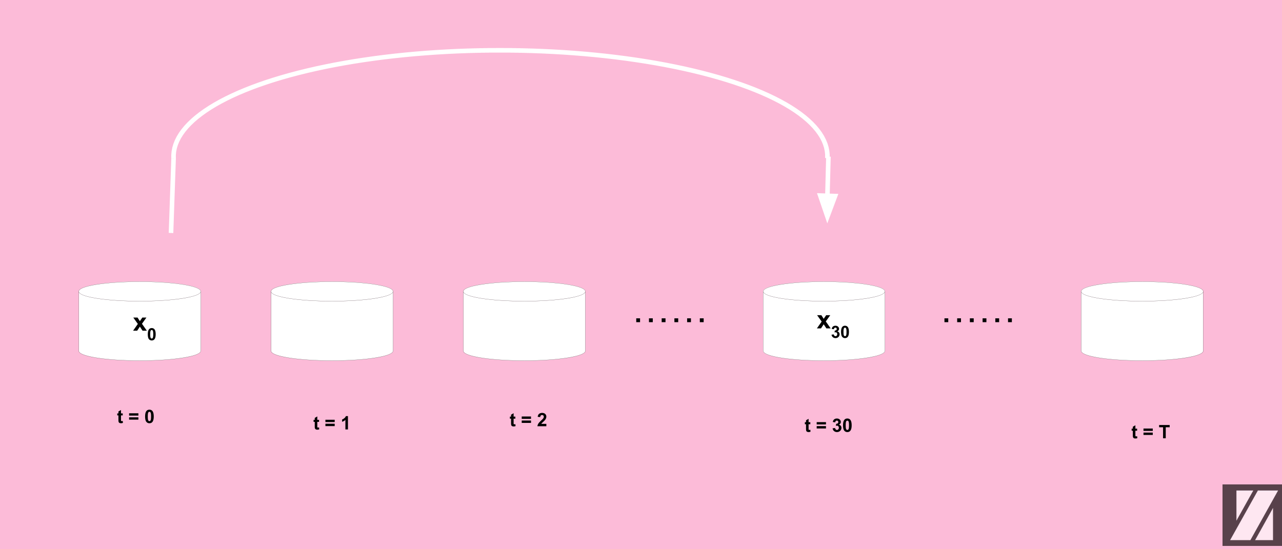
Suppose that we want to perturb x over T = 50, and we want to get the noisy input sample x, but without the need to calculate it overall T, how can we do that?
The Reparametrization Trick allows us to change a stochastic process to a deterministic process. Here it helps us to to jump over several time steps in one single operation to update x. In other words:
This means that to get the noisy version of x at T = t, we need to multiply the input sample x by a term called signal rate, then add it to a standard Gaussian noise which is multiplied by a term called noise rate.
Here is the mathematical definition of these terms:
The product of all alpha from t = 0 to t = t is defined as:
The noise rate is:
The signal rate is:
Where:
If these equations are not clear to you or you don’t know what is the reparameterization trick, don’t worry! we will have other posts that discuss these concepts in detail.
5.1.3 Diffusion Schedule

A diffusion schedule is a technique that describes how the values of:
beta change with t. At the early stage of the nosing process, we use smaller values of beta then we start to increase it with time.
There are multiple ways to apply the scheduling during the diffusion process, here are some of the used methods:
Linear Diffusion Schedule: In this type of schedule the values of beta over all the time steps T are generated in a linear way, where the range of these values usually falls in the range [0.0001 - 0.02]. This means, the noising process will have a linear form during the diffusion operation:
\(\beta_t \in [10^{-4}, 0.02]\)Cosine Diffusion Schedule: Cosine scheduling achieved a better performance compared to linear scheduling in [Alex et al]. Here is the formula used to update x during the T timesteps:
\(\begin{array} {lcl} \bar \alpha_t &= &\frac{f(t)}{f(0)} \\ f(t) &=& cos(\frac{t }{T} . \frac{\pi}{2})^2 \end{array}\)Offset-Coine Diffusion Schedule: This is similar to the cosine diffusion schedule, except that we will add a small number to the equation to prevent Beta from being too small at t = 0.
5.2 Reverse Process

The goal of the reverse process is to:
Predict the total amount of noise that was injected into a given input sample through the forward process.
To do that, It uses the following components:
5.2.1 Sinusoidal Embedding
Its other name is positional encoding — It is a type of embedding that is used to convert a scalar number to a continuous vector representation. The reverse process uses this embedding component to convert the noise rate to a continuous vector representation that the UNet model can process.
where:
For example for an embedding vector with size = 32, L = 16.
The function f is defined as:
5.2.2 UNet Model
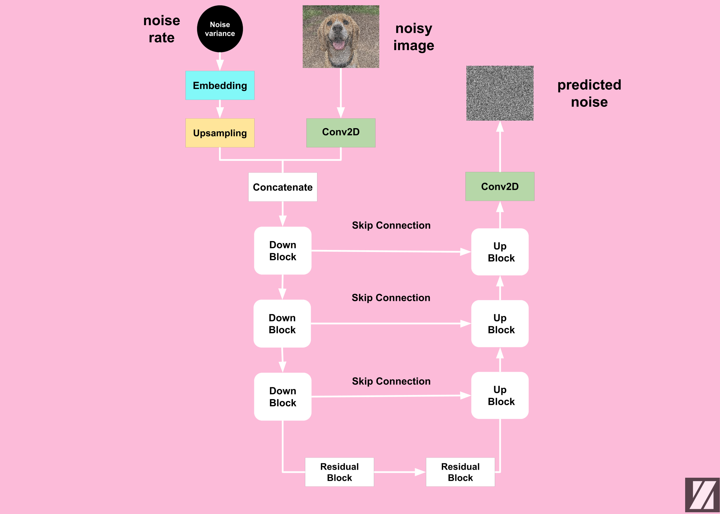
The UNet is a popular architecture in computer vision for image segmentation tasks. Diffusion models use it for performing a regression task to predict the total amount of noise that has been added to a noisy sample. It consists of the following components:
Upsampling Block: To increase the spatial dimension of the noise variance vector.
Convolution Block: To increase the number of channels of the input sample.
DownBlock: To compress the input sample spatially and expand channel-wise.
UpBlock: To expand the input sample in the spatial dimension while reducing the channel dimension.
Residual Block: To mitigate the vanishing gradient problem during the training process.
Skip Connection Block: To allow the information to shortcut parts of the network and flow through to later layers.
6. Recap
In this article, we've explored Denoising Diffusion Models (DDMs). We've highlighted their importance, delved into how they work, and examined their architecture, focusing on the Forward and Reverse Processes.
We've discussed key components like the Diffusion Schedule, Sinusoidal Embedding, and UNet Models. It's worth noting that Diffusion Models bring advantages in terms of sample quality and inference time.
7. References
Jonathan Ho, Ajay Jain, and Pieter Abbeel. "Denoising Diffusion Probabilistic Models" (2020).
Alex Nichol and Prafulla Dhariwal. "Improved Denoising Diffusion Probabilistic Models" (2021).
Yang Song, Jascha Sohl-Dickstein, Diederik P. Kingma, Abhishek Kumar, Stefano Ermon, and Ben Poole. "Score-Based Generative Modeling through Stochastic Differential Equations" (2021).
Jascha Sohl-Dickstein, Eric A. Weiss, Niru Maheswaranathan, and Surya Ganguli. "Deep Unsupervised Learning using Nonequilibrium Thermodynamics" (2015).
David Foster's "Generative Deep Learning, 2nd Edition" (2023).
Before Goodbye!

Want to Cite this Article?
@article{khamies2023denoising,
  title   = "Denoising Diffusion Models (DDMs) under the Microscope",
  author  = "Waleed Khamies",
  journal = "Zitoon.ai",
  year    = "2023",
  month   = "Aug",
  url     = "https://publication.zitoon.ai/denoisng-diffusion-models-ddms-under-the-microscope"
}
New to this Series?
New to the “Generative Modeling Series”? Here you can find the previous articles in this series [link to the full series].
Any oversights in this post?
Please report them through this Feedback Form, we really appreciate that!
Thank you for your reading!
Thank you for your reading! If you would like to receive the next posts in this series in your email, please feel free to subscribe to the ZitoonAI Newsletter. Come and Join the Family!