From Meaning to a Noise: Inside the Forward Process of Diffusion Models (DDMs)

A Closer Look into the Noise Process of DDMs.

Aug 30, 2023

The Forward Process of the Diffusion Model.

Table of Content

Introduction.
Notations.
Problem Definition.
The Unreparameterized Forward Process.
Reparametrization Trick.
The Reparameterized Forward Process
1. Merging Two Gaussian Distributions.
2. The Equation.
Diffusion Schedule
1. Linear Schedule.
2. Cosine Schedule.
3. Offset-Cosine Schedule.
Recap.
References.

1. Introduction

In the last post, we briefly discussed denoising diffusion models (DDMs). We learned that the diffusion model is a type of generative model that tries to learn the distribution of data by modeling the data generation using a denoising process. Also, we knew the main components of the diffusion models, and how the forward process and reverse process help us to generate a novel sample from a completely random noise.

Today, we will address the forward process component in detail. We will learn how the diffusion models will transform a meaningful input into a random noise through a sequential process to learn a data distribution and generate novel samples. First, we will explain the forward process by defining the problem. Then, we will talk about an important trick that is used in Bayesian statistics to handle stochastic processes.

After that, we will derive the main equation of the forward process. Finally, we will talk about an important technique that helps in optimizing the performance of the diffusion models and minimizing the reverse process objective function, the diffusion schedule. Let’s dive in!

2. Notations

\( \begin{array}{lcl} x &\equiv& \text{A data point} \\ d &\equiv& \text{A real data distribution.}\\ q &\equiv& \text{The forward process function (Gaussian distribution function.} \\ \beta_t &\equiv& \text{The noise variance at arbitrary step t.} \\ \alpha_t &\equiv& \text{The noise variance at arbitrary step t.} = 1- \beta_t \\ \bar \alpha_t &\equiv& \text{The noise variance schedule at arbitrary step t.} = \prod^t_{i=0} \alpha_i \\ \bar \alpha_t &\equiv& \text{The signal rate at arbitrary step t.} \\ 1-\bar \alpha_t &\equiv& \text{The noise variance rate at arbitrary step t.} \end{array}\)

3. Problem Definition

3.1 In Words

The process of adding a small amount of noise to a sample gradually over many steps until the sample is converted to completely standard Gaussian noise.

3.2 In Math

Let’s assume that we have a data point x that is sampled from a distribution d and we want to perturb it by adding a noise ε sampled from a Gaussian distribution N(0, I) over T steps. The variances of the noisy samples over the T steps:

\(x = [ x_0, x_1, x_2, ..., x_T]\)

are provided by a scheduler S :

\(S = [\beta_t \in {(0,1)}]^T_{t=1} \)

For example S = [0.001, 0.03, 0.34 ] for T =3.

4. The Unreparameterized Forward Process

Given that we have a function q that adds a small amount of Gaussian noise to a data point x over T steps, we can define the mathematical form of q as follows (Eq1):

\(q(x_t | x_{t-1}) = \mathcal{N}(x_t | \sqrt {1-\beta_t} x_{t-1} , \beta_t I)\)

where:

\(\mathcal{N} \equiv \text{Gaussian Distribution}\)

\(\sqrt {1-\beta_t} x_{t-1} \equiv \text{The mean.}\)

\(\beta I \equiv \text{The variance.}\)

Also, we should note that q is a Gaussian distribution. So if we want to express the joint probability of all the values of x over T steps, we can express it as the product of conditional probabilities:

\(q(x_1, x_2, x_3, ..., x_T | x_0 ) = \prod^T_{t=1} q(x_t | x_{t-1}) \)

5. Reparametrization Trick

The previous equation of the forward process can be written in a much simpler way. Suppose that we want to calculate the noisy sample of x at a step t = 25 but without calculating all the values from t = 1 to t = 25. In other words, we want to be able to calculate that in just one operation (Jumping directly to t = 25).

The parameterization trick can help us to do that. But before jumping to see the simpler version of the forward process equation, let’s explain briefly what the reparameterization trick is.

The parameterization trick is a technique used in Bayesian statistics to express a stochastic random variable z as a deterministic variable.

Mathematically, the stochastic form of z is:

\(z \sim \mathcal q(z|x, \phi)\)

The parameterization trick will help us to express it in a deterministic form:

\(z = g(x, \phi)\)

Why do we want to do that?

Suppose that we want to optimize the q function with respect to its parameters(i.e. Φ). We can’t do this optimization, and find the best values of the parameters that produced the best output for that q function.

This is because of the sampling process nature. It is a stochastic operation that can’t be differentiated. Each time we call the function q above, it will give us a different value due to the randomness of the sampling operation itself. This makes calculating the gradient of this function undefined.

Therefore, to be able to calculate the gradients, the parameterization trick helps us to change the stochastic operation to a deterministic operation by decoupling the stochasticity from the main equation as follows:

\(g(x, \phi) = \mu + \sigma * \epsilon\)

where:

\(\epsilon \sim \mathcal N(0, I)\)

As we can see, now the epsilon is sampled from a standard Gaussian distribution, and then added to the equation as a constant. This simple trick helps the gradient of a loss function f to be calculated with respect to the parameters (i.e. Φ). Here is a visual illustration of that:

The Reparameterization Trick. ( by Kingma & Welling, NIPS workshop 2015)

6. The Reparameterized Forward Process

6.1 Merging Two Gaussians Distributions

In statistics, we learned that if we have two Gaussian distributions:

\(\begin{array}{lcl} G_1 &=& \mathcal N(\mu_1, \sigma^2_{1}I) \\ G_2 &=& \mathcal N(\mu_2, \sigma^2_{2}I) \end{array}\)

If we want to merge or combine them G = G1 + G2, we can do the following:

The new mean will be:

\(\mu_{merged} = \frac{w_1 * \mu_1 + w_2 * \mu_2}{w_1 + w_2}\)

And the new variance will be:

\(\sigma^2_{merged} = \frac{w_1 * \sigma^2_1 + w_2 * \sigma^2_2}{w_1 + w_2}\)

w1 and w2 are parameters that control how much contribution we want from each distribution.

In the case of standard Gaussian distributions, where the mean is zero and the variance is 1 or the identity vector, the mean and variance of the merged distributions will be:

\(\mu_{merged} = 0\)

\(\sigma^2_{merged} = \sigma^2_1 + \sigma^2_2\)

6.2 The Reparameterized Forward Process

Let’s jump back to see how the reparameterization trick helps us to get a close form of the previous forward process equation. Here, the trick is used to get a close form, and not to mainly simplify the gradient flow as we saw in the previous section.

The previous equation (Eq1):

\(q(x_t | x_{t-1}) = \mathcal{N}(x_t | \sqrt {1-\beta_t} x_{t-1} , \beta_t I)\)

is expressed using the parameterization trick using a deterministic equation as follows (Eq 3):

\(\begin{array}{lcl} x_t &=& C_1 x_{t-1} + C_2 * \epsilon_{t-1} \\ \\ \textbf{where:} \\ C_1 &=& \sqrt{1-\beta_t} = \mu \\ C_2 &=& \sqrt{\beta_t} = \sigma \\ \epsilon_{t-1} &\sim& \mathcal N(0, I) \end{array}\)

Now, given the deterministic equation, let’s derive the close form of the forward process by defining some important variables:

Alpha

\(\alpha_t = 1- \beta_t\)

Alpha Product

The product of alpha(s) in all the steps from i = 0 to i = t can be expressed as:

\(\overline \alpha_t = \prod^{t}_{i=0} \alpha_i\)

Now, let’s calculate the value of x at step = t-1 (Eq 4)

\(x_{t-1} = \sqrt{\alpha_{t-1}} \space x_{t-2} + \sqrt{1-\alpha_{t-1}} \space \epsilon_{t-2}\)

Let’s substitute that in (Eq3) as follows:

Now, let’s use the merging property of the two Gaussians where:

\(\begin{array}{lcl} G_1 &=& \sqrt{\alpha_t} \textcolor{red}{ \sqrt{1-\alpha_{t-1}} \space \epsilon_{t-2}} \\ \mu_1 & = & 0\\ \sigma^2_1 &=& \sqrt{\alpha_t} \sqrt{1-\alpha_{t-1}} \end{array} \)

\( \begin{array}{lcl} G_2 &=& \sqrt{1-\alpha_t} \space \epsilon_{t-1} \\ \mu_1 & = & 0\\ \sigma^2_1 &=& \sqrt{1-\alpha_{t}} \end{array}\)

\(G_{merged} = \mathcal N (\mu_{merged}, \sigma_{merged})\)

Given that, they are standard Gaussian distributions:

\(\mu_{merged} = 0\)

\(\begin{array} {lcl} \sigma^2_{merged} &=& \sqrt{\alpha_t} \sqrt{1-\alpha_{t-1}} + \sqrt{1-\alpha_t} \\ & = &\sqrt{\alpha_t (1-\alpha_{t-1}) +1-\alpha_t } \\ & = & \sqrt{\alpha_t - \alpha_t \alpha_{t-1} +1-\alpha_t } \\ & = & \sqrt{1 - \alpha_t \alpha_{t-1} } \end{array}\)

Now, (Eq3) will be transformed as follows:

Where:

\(\bar \epsilon_{t-2} = G_{merged}\)

Now, if we keep the substitution, we could notice the pattern of Alpha Product:

\(\begin{array} {lcl} x_t & = &\sqrt{\alpha_t} \space x_{t-1} + \sqrt{1-\alpha_t} \space \epsilon_{t-1} \\ & = & \sqrt{\alpha_t} \textcolor{red}{ [\sqrt{\alpha_{t-1}} \space x_{t-2} + \sqrt{1-\alpha_{t-1}} \space \epsilon_{t-2}] }+ \sqrt{1-\alpha_{t}} \space \epsilon_{t-1} \\ & = & \textcolor{green}{\sqrt{\alpha_t \alpha_{t-1}}} \space x_{t-2} + \sqrt{1 - \textcolor{green}{\alpha_t \alpha_{t-1} }} \bar \epsilon_{t-2} \\ & = & \textcolor{green}{\sqrt{\alpha_t \alpha_{t-1}\alpha_{t-2}}} \space x_{t-3} + \sqrt{1 - \textcolor{green}{\alpha_t \alpha_{t-1}\alpha_{t-2} }} \bar \epsilon_{t-3} \\ & = & \underbrace{\textcolor{green}{\sqrt{\alpha_t \alpha_{t-1}\alpha_{t-2} \alpha_{t-3}}}}_{\bar \alpha_3} \space x_{t-4} + \sqrt{1 - \underbrace{\textcolor{green}{\alpha_t \alpha_{t-1}\alpha_{t-2} \alpha_{t-3} }}_{\bar \alpha_3}} \bar \epsilon_{t-4} \\ &=& ... \end{array}\)

Then, if we keep the expansion till t = 0, then (Eq3) will be as follows:

\(\begin{array} {lcl} x_t & = &\sqrt{\alpha_t} \space x_{t-1} + \sqrt{1-\alpha_t} \space \epsilon_{t-1} \\ & = & \sqrt{\alpha_t} \textcolor{red}{ [\sqrt{\alpha_{t-1}} \space x_{t-2} + \sqrt{1-\alpha_{t-1}} \space \epsilon_{t-2}] }+ \sqrt{1-\alpha_{t}} \space \epsilon_{t-1} \\ & = & \textcolor{green}{\sqrt{\alpha_t \alpha_{t-1}}} \space x_{t-2} + \sqrt{1 - \textcolor{green}{\alpha_t \alpha_{t-1} }} \bar \epsilon_{t-2} \\ & = & \textcolor{green}{\sqrt{\alpha_t \alpha_{t-1}\alpha_{t-2}}} \space x_{t-3} + \sqrt{1 - \textcolor{green}{\alpha_t \alpha_{t-1}\alpha_{t-2} }} \bar \epsilon_{t-3} \\ &=& ... \\ & = & \textcolor{green}{\sqrt{\alpha_t \alpha_{t-1}\alpha_{t-2} \alpha_{t-3}...\alpha_{t-{T+5}}}} \space x_{t-{T+6}} + \sqrt{1 - \textcolor{green}{\alpha_t \alpha_{t-1}\alpha_{t-2} \alpha_{t-3}......\alpha_{t-{T+5}}}} \bar \epsilon_{t-{T+6}} \\ &=& ... \\ & = & \sqrt{\bar \alpha_t} \space x_{0} + \sqrt{1- \bar \alpha_t} \space \epsilon \end{array} \)

And this is the close form of the forward process (Eq4):

\(\begin{array}{lcl} x_t &=& \sqrt{\bar \alpha_t} \space x_{0} + \sqrt{1- \bar \alpha_t} \space \epsilon \\ \\ \textbf{where:} \\ x_t &=& \text{The noisy input sample after arbitrary t time step.} \\ x_0 &=& \text{The ground-truth (not noisy) input sample (i.e. image)} \\ \overline \alpha_t &=& \prod^{t}_{i=0} \alpha_i \\ \epsilon &\sim& \mathcal N(0,1) \end{array}\)

7. Diffusion Schedule

A diffusion schedule is a technique that describes how the values of beta change with t.

At the early stage of the nosing process, we use smaller values of beta then we start to increase it with time.

There are multiple ways to apply the scheduling during the diffusion process, here are some of the popular methods:

Linear Diffusion Schedule: In this type of schedule the values of beta over all the time steps T are generated linearly, where the range of these values usually falls in the range [0.0001 - 0.02]. This means, the noising process will have a linear form during the diffusion operation:
\(\beta_t \in [10^{-4}, 0.02]\)
Cosine Diffusion Schedule: Cosine scheduling achieved a better performance compared to linear scheduling [Nichol & Dhariwal]. Here is the formula used to update x during the T timesteps:
\(\begin{array} {lcl} \bar \alpha_t &= &\frac{f(t)}{f(0)} \\ f(t) &=& cos(\frac{t }{T} . \frac{\pi}{2})^2 \end{array}\)
Offset-Coine Diffusion Schedule: This is similar to the cosine diffusion schedule, except we will add a small number of s to the equation to prevent beta from being too small at t = 0.
\(\begin{array} {lcl} \bar \alpha_t &= &\frac{f(t)}{f(0)} \\ f(t) &=& cos(\frac{t/T + s}{1+s} . \frac{\pi}{2})^2 \end{array}\)

Note
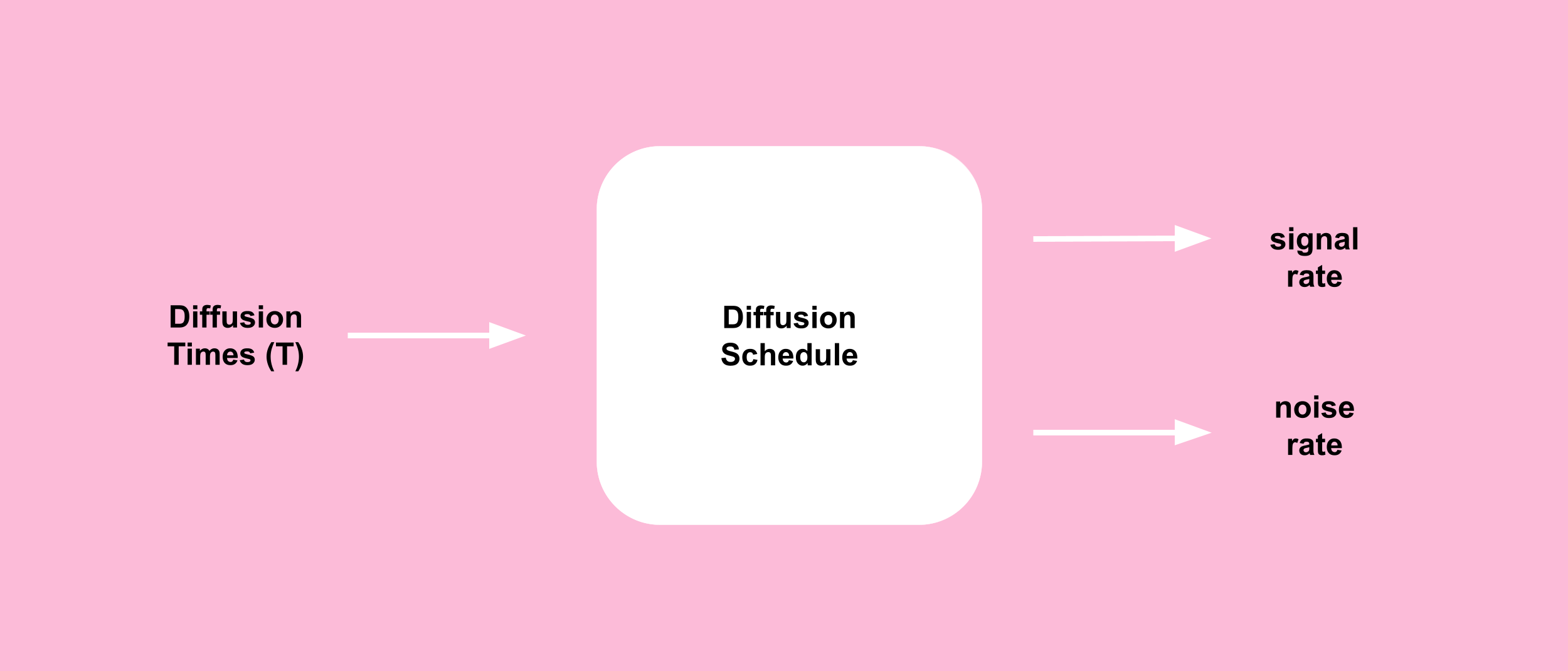
You could notice that in the image above the diffusion schedule component outputs two values: 1) The signal rate, and 2) The noise rate, as we need these values in the forward proces equation (Eq4).
We defined these values in the “Notations” section above, but here is another reminder for you:
\(\begin{array}{lcl} \\ \bar \alpha_t &\equiv& \text{The signal rate at arbitrary step t.} \\ 1-\bar \alpha_t &\equiv& \text{The noise variance rate at arbitrary step t.} \end{array}\)

The next figure shows the difference in performance between linear scheduling and cosine scheduling during the training process:

Linear Scheduling vs. Cosine-based Scheduling. (by Nichol et al., 2021)

Your Takeaway From This Post

photo of bulb artwork — Photo by AbsolutVision on Unsplash

The Forward Process Equation For Denoising Diffusion Models (DDMs) is:

\(\begin{array}{lcl} x_t &=& \sqrt{\bar \alpha_t} \space x_{0} + \sqrt{1- \bar \alpha_t} \space \epsilon \\ \\ \textbf{where:} \\ x_t &=& \text{The noisy input sample after arbitrary t time step.} \\ x_0 & \equiv& \text{The ground-truth (not noisy) input sample (i.e. image)} \\ \overline \alpha_t &\equiv& \text{Signal rate}= \prod^{t}_{i=0} \alpha_i \\ 1- \overline \alpha_t & \equiv& \text{Noise rate} \\ \epsilon &\sim& \mathcal N(0,1) \end{array}\)

8. Recap

In this post, we talked about the forward process in denoising diffusion models (DDMs). This is how we turn meaningful data into random noise.
We started by defining the forward process and showing how to express it in math.
We also introduced a useful trick from Bayesian statistics that helps us to obtain the closed form of the forward process.
Then, we showed you the main equation that describes how the forward process works mathematically.
Finally, we talked about the diffusion schedule, which describes how the values of beta change with t.

See You Soon!

9. References

Jonathan Ho, Ajay Jain, and Pieter Abbeel. "Denoising Diffusion Probabilistic Models" (2020).
Alex Nichol and Prafulla Dhariwal. "Improved Denoising Diffusion Probabilistic Models" (2021).
David Foster's "Generative Deep Learning, 2nd Edition" (2023).
Lilian Weng. "What are Diffusion Models?" (2021). Lilian Weng's Blog
Lilian Weng. "Reparameterization Trick - From Autoencoder to Beta-VAE" (2018).

Want to Cite this Article?

@article{khamies2023meaning,
  title   = "From Meaning to a Noise: Inside the Forward Process of Diffusion Models (DDMs)",
  author  = "Waleed Khamies",
  journal = "Zitoon.ai",
  year    = "2023",
  month   = "Aug",
  url     = "https://publication.zitoon.ai/from-meaning-to-a-noise-inside-the-forward-process-of-diffusion-models"
}

New to this Series?

New to the “Generative Modeling Series”? Here you can find the previous articles in this series [link to the full series].

Any oversights in this post?

Please report them through this Feedback Form, we really appreciate that!

green and black animal plush toy — Photo by JOSHUA COLEMAN on Unsplash

Thank you for your reading!

Thank you for your reading! If you would like to receive the next posts in this series in your email, please feel free to subscribe to the ZitoonAI Newsletter. Come and Join the Family!